Replies

"what does 1750 data have to do with doing a curve fit against spectral data?

The eq.

F_CO₂ = 5.35ln(C/C_o) = watts absorbed above the 278ppmv baseline from 1750.

That's my understanding of it. Note that at C=C_o, the watts = 0. The eq is an equivalent to Beer's law:
I=I_o(1-e^{- α *c*x}) , where α is the absorbtion coefficient, c is the baseline concentration, and x is the pathlength. The eq. is then used to find F_CO₂ above 1750's value.

F_CO₂ = I_now - I₁₇₅₀ = I₁₇₅₀(e^{- α *xc₁₇₅₀} - e^{- α *xc_now}).

Each molecule can absorb at many wavelengths, and each has it's own transition probability. So, the exponential terms are of the form Σ_n e^{- α_n *xc}.

F_CO₂ = I₁₇₅₀( Σ_ne^{- α_n *xc₁₇₅₀} - Σ_ne^{- α_n *xc_now}).

You can see the constants in there. I assume Myhre considered this as a change in intensity due to the probability of more excited states with a change in concentration, dE_excited = A*dc/C. I= A*ln(C/C_o), where A represents some sum of absorbtion constants, as above. Fitting obtains, 5.35ln(C/C₁₇₅₀). Then F_CO₂=I.

At any particular instant, there will be a population of excited molecules. They will decay and reradiate in another direction, they will scatter radiation, and they will decay by transfer of kinetic energy to the surounding gas. The caption to the graph you showed me, then provided a link for says, "The graph at left shows the percentage of energy absorbed in a clear tropical sky by water vapor (green) and carbon dioxide (brown)." In order to absorb 100% of the radiation, there must be unexcited molecules with states available.

"There are more CO2 molecules than there are photons of IR at the proper wavelengths to be absorbed in a given path length of atmosphere.

If that were true, then the caption on that figure could never say 100%. It would have to say something less.

" Increasing concentration effectively broadens the spectral line allowing more absorption by weak lines and the skirts either side of the central spectral line which are not saturated.

Increasing concentration provides more unexcited molecules to absorb radiation. More States are available. The width of those lines around a vibration is due to rotational coupling with the vibration and dopler spreading. The wavelength must match for any particular combo of vibration, rotation and molecular velocity. It is less probable that those vibrations with other angular momentum will be excited. The angular momnetum is coupled, so the vibrational E changes and has max values at J=0 and in the p and r branches, about 4 Δ Js away from there. That's why their peaks are successively lower as the wavelength moves from the base vibrational wavelength. The pressure broadening should be constant.

F_CO_₂ = 5.35ln(C/C_o) = watts absorbed above the 278ppmv baseline from 1750.
That's my understanding of it. Note that at C=C_o, the watts = 0.

Actually, Co can be any base you want to apply within the log functions it's effective range, it is not limited to Co=285. It is just as accurate at Co=185ppmv doubling to 390ppmv, as it would be at Co = 500ppmv doubling to 1000ppmv.

It is a general empirical relationship derived from spectroscopic Line by Line integrations.

The eq is an equivalent to Beer's law

Only in a very general sense as Beer's law holds valid for only very low concentrations for a specified monochromatic wavelength where absorption is a linear function of concentrations (e.g. <10ppmv for CO2 in my experience.

refer here for some basics on the applicability of Beer's Law: http://teaching.shu.ac.uk/hwb/chemistry/tutorials/molspec/beers1.htm

A = ebc tells us that absorbance depends on the total quantity of the absorbing compound in the light path through the cuvette. If we plot absorbance against concentration, we get a straight line passing through the origin (0,0).

Note that the Law is not obeyed at high concentrations. This deviation from the Law is not dealt with here.

The linear relationship between concentration and absorbance is both simple and straightforward, which is why we prefer to express the Beer-Lambert law using absorbance as a measure of the absorption rather than %T.

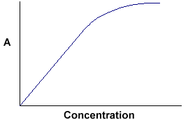
At higher concentrations, you approach extinction levels and the relationship breaks down very rapidly.

When you deal in multiple lines at differing strengths and different places in the blackbody radiance curve it becomes nearly a logarithmic function at moderately high concentration and ultimately going to full extinction in the extreme cases of very high concentrations where even weak lines are at extinction levels for the illumination intensities associated with blackbody radiation.

Each molecule can absorb at many wavelengths, and each has it's own transition probability. So, the exponential terms are of the form S_n e^{- a}n^*xc.

Correct, which would require a Line-by-Line integration with respect to blackbody curve and the multitude of wavelengths involved for high accuracy. Or one may choose to do the Line-By-Line integrations necessary and do a curve fit for the range of concentrations and wavelengths of interest deriving an empirical relationship for general use, which is what the Myhre relation does.

When near extinction levels for the flux levels associated with 200-300K blackbody radiation and multiple lines come into with differing strengths and multiple wavelengths you need a more general approach if you are not going to do Line-by-Line integrations for your calculations for every change in concentration, which can be a computationally expensive approach to modeling. Under such conditions you will find that the overall absorption relation passes through a log response in the 100-2800 ppmv range of concentrations.

An example is the dominant absorption band of 12-18um for CO2:

Given dC is some fraction 320ppmv, i.e. (Concentration-320)/320 for the particular instance

the strong line absorption at its band of wavelengths in the 288K blackbody spectrum fits,

DFw/m²= 12.6 * (1-e^-9.65x10^{^-4*}^d^C)

plotting a strongly limiting function,

While weakline responses elsewhere in the 288K black body spectrum fits

DF w/m² = 11.9 * (1-e^-2.22x10^{^-4*}^d^C)

plotting out as a near linear response up to very high CO2 concentrations

Take the sum of them and you will find that a log relationship can be fit through a significant portion of the curve at concentrations around present day CO2 levels for a representative broad band response, rather than at the limited monochromatic single line response for which Beer's law is generally applied.

Refer to

A Radiative-Convective Model Study of the CO2 Climate Problem
Augustssona & Ramanathan (1977),
Journal of the Atmospheric Sciences, Vol. 34 Issue 3, pp. 448–451 Refer: page 450, Figure 3

For a discussion of how such is applied in a simple model representing climate responses.

Increasing concentration provides more unexcited molecules to absorb radiation. More States are available.

And the effect of that is different from saying:

Increasing concentration effectively broadens the spectral line allowing more absorption by weak lines and the skirts either side of the central spectral line which are not saturated.

how?

The point being that one does not always wish to do full line-by-line integrations for empirical work, especially not when one wants a view of how the whole changes across a range of interest and an empirical relation serves well within known error range. 5% accuracy for an function will do quite well when your other variables are essentially stabs in the dark with estimation errors of 20-100%are the rule as in today's flock of GCMs.

Radiative forcing by well-mixed greenhouse gases:
Estimates from climate models in the
Intergovernmental Panel on Climate Change
(IPCC) Fourth Assessment Report (AR4)
http://www.agu.org/pubs/crossref/2006.../2005JD006713.shtml
http://pubs.giss.nasa.gov/abstracts/2006/Collins_etal.html
http://pubs.giss.nasa.gov/docs/2006/2006_Collins_etal.pdf

Collins, W.D., V. Ramaswamy, M.D. Schwarzkopf, Y. Sun, R.W. Portmann, Q. Fu, S.E.B. Casanova, J.-L. Dufresne, D.W. Fillmore, P.M.D. Forster, V.Y. Galin, L.K. Gohar, W.J. Ingram, D.P. Kratz, M.-P. Lefebvre, J. Li, P. Marquet, V. Oinas, Y. Tsushima, T. Uchiyama, and W.Y. Zhong 2006. Radiative forcing by well-mixed greenhouse gases: Estimates from climate models in the Intergovernmental Panel on Climate Change (IPCC) Fourth Assessment Report (AR4). J. Geophys. Res. 111, D14317, doi:10.1029/2005JD006713.
The radiative effects from increased concentrations of well-mixed greenhouse gases (WMGHGs) represent the most significant and best understood anthropogenic forcing of the climate system. The most comprehensive tools for simulating past and future climates influenced by WMGHGs are fully coupled atmosphere-ocean general circulation models (AOGCMs). Because of the importance of WMGHGs as forcing agents it is essential that AOGCMs compute the radiative forcing by these gases as accurately as possible. We present the results of a radiative transfer model intercomparison between the forcings computed by the radiative parameterizations of AOGCMs and by benchmark line-by-line (LBL) codes. The comparison is focused on forcing by CO₂, CH₄, N₂O, CFC-11, CFC-12, and the increased H₂O expected in warmer climates. The models included in the intercomparison include several LBL codes and most of the global models submitted to the Intergovernmental Panel on Climate Change (IPCC) Fourth Assessment Report (AR4). In general, the LBL models are in excellent agreement with each other. However, in many cases, there are substantial discrepancies among the AOGCMs and between the AOGCMs and LBL codes. In some cases this is because the AOGCMs neglect particular absorbers, in particular the near-infrared effects of CH₄ and N₂O, while in others it is due to the methods for modeling the radiative processes. The biases in the AOGCM forcings are generally largest at the surface level. We quantify these differences and discuss the implications for interpreting variations in forcing and response across the multimodel ensemble of AOGCM simulations assembled for the IPCC AR4.

Comparative results of this study show the relative contributions of H2O & CO2 to the anthropogenic global warming hypothesis under IPCC scenarios using the IPCC suite of AOGCMs used in the of their coming AR4 report.

vs the H2O column water vapor increase of 20%.

demonstrating the positive feedback dependency of the models as well as the forcing that each contributes in a relative comparison. Note the more than 20 to 1 forcing of water vapor over CO2 at the surface where global climate change has its most meaningful effect on us poor surface dwelling creatures.

Dang, dropped the graphics on me. Try that last reference with real URL's instead of my harddrive this time:

Radiative forcing by well-mixed greenhouse gases:
Estimates from climate models in the
Intergovernmental Panel on Climate Change
(IPCC) Fourth Assessment Report (AR4)
http://www.agu.org/pubs/crossref/2006.../2005JD006713.shtml
http://pubs.giss.nasa.gov/abstracts/2006/Collins_etal.html
http://pubs.giss.nasa.gov/docs/2006/2006_Collins_etal.pdf

Collins, W.D., V. Ramaswamy, M.D. Schwarzkopf, Y. Sun, R.W. Portmann, Q. Fu, S.E.B. Casanova, J.-L. Dufresne, D.W. Fillmore, P.M.D. Forster, V.Y. Galin, L.K. Gohar, W.J. Ingram, D.P. Kratz, M.-P. Lefebvre, J. Li, P. Marquet, V. Oinas, Y. Tsushima, T. Uchiyama, and W.Y. Zhong 2006. Radiative forcing by well-mixed greenhouse gases: Estimates from climate models in the Intergovernmental Panel on Climate Change (IPCC) Fourth Assessment Report (AR4). J. Geophys. Res. 111, D14317, doi:10.1029/2005JD006713.
The radiative effects from increased concentrations of well-mixed greenhouse gases (WMGHGs) represent the most significant and best understood anthropogenic forcing of the climate system. The most comprehensive tools for simulating past and future climates influenced by WMGHGs are fully coupled atmosphere-ocean general circulation models (AOGCMs). Because of the importance of WMGHGs as forcing agents it is essential that AOGCMs compute the radiative forcing by these gases as accurately as possible. We present the results of a radiative transfer model intercomparison between the forcings computed by the radiative parameterizations of AOGCMs and by benchmark line-by-line (LBL) codes. The comparison is focused on forcing by CO₂, CH₄, N₂O, CFC-11, CFC-12, and the increased H₂O expected in warmer climates. The models included in the intercomparison include several LBL codes and most of the global models submitted to the Intergovernmental Panel on Climate Change (IPCC) Fourth Assessment Report (AR4). In general, the LBL models are in excellent agreement with each other. However, in many cases, there are substantial discrepancies among the AOGCMs and between the AOGCMs and LBL codes. In some cases this is because the AOGCMs neglect particular absorbers, in particular the near-infrared effects of CH₄ and N₂O, while in others it is due to the methods for modeling the radiative processes. The biases in the AOGCM forcings are generally largest at the surface level. We quantify these differences and discuss the implications for interpreting variations in forcing and response across the multimodel ensemble of AOGCM simulations assembled for the IPCC AR4.

:
Comparative results of this study show the relative contributions of H2O & CO2 to the anthropogenic global warming hypothesis under IPCC scenarios using the IPCC suite of AOGCMs used in the of their coming AR4 report.

vs the H2O column water vapor increase of 20%.

demonstrating the positive feedback dependancy of the models as well as the forcing that each contributes in a relative comparison. Note the more than 20 to 1 forcing of water vapor over CO2 at the surface where global climate change has its most meaningful effect on us poor surface dwelling creatures.